datarich(ard)
a personal journey into data science
Bayesian partial pooling shrinkage magic
by datarich(ard)
Partial pooling
A Bayesian model provides a cohorent and succinct expression of mixed-effects in multilevel models, in which individual variation can be treated skeptically and appropriately as a deviation from the wider population. This means individual-level effects will be more or less partially shrunk to the population depending upon the posterior probability of the model. This allows us to describe individual responses in an appropriately scaled (and skeptical) fashion when they deviate from the population norm.
Such models represent the variation in each cluster (individual) as well as the variation in the wider population. Depending upon the variation among clusters, which is learned from the data as well, the model pools information across clusters. This pooling tends to improve estimates about each cluster. This has several pragmatic benefits:
- Improved estimates for repeated sampling
- Improved estiamtes for inbalanced in sampling
- Explicit estimates of variation
- Avoids averaging and retains information
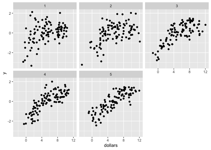
This document compares partial pooling, full pooling and no pooling in the context of a piecewise regression model, where we are interested in determining the change-point or inflection point in the relationship between two variables (e.g., income and happiness).
Data generation
Because this is a simulation, we can define the data generating process:
Yit = β0 + β1(xit - ωt)(xit < ωt) + β2(xit - ωt)(xit ≥ ωt)
Where:
i is the individual
t is the year
β0 is our intercept
β1 is the slope prior to inflection point
β2 is the slope after the inflection point
ωt is the location of the inflection point on the x-scale
(e.g., income) for each year (t)
In our case, ω will vary over clusters (years) and we want to find the true location of ω for each cluster/year. The data is generated by the above formula, where β0 = 0, β1 = 1, β2 = 0, and ωt..5 = 3, 4, 5, 6, 7.
Models
No pooling
In brms, we will define the following model with a fixed intercept for alpha for each year (alpha is the rescaled ω parameter). This is our no pooling model because the model does not share information for alpha between years, i.e., there is no population-level estimate for alpha with which to learn from or provide shrinkage. (The other parameters, b0, b1, & b2 have both population- and group-level intercepts, i.e., “partial pooling”):
np_formula <- bf(
  y ~ b0 + b1 * (dollars - omega) * step(omega - dollars) +
    b2 * (dollars - omega) * step(dollars - omega),
  b0 + b1 + b2 ~ 1 + (1|year), # fixed for all years, random each year
  alpha ~ 0 + year, # single fixed intercept for each year (i.e., no pooling)

  # Sigmoid transform to keep omega within the range of 0 to x
  nlf(omega ~ inv_logit(alpha) * 10),
  nl = TRUE
)
Because it is a nonlinear model (nl = TRUE), we will need to
explicitly define our priors:
# priors
bprior <- prior(normal(0, 3), nlpar = "b0") +
  prior(normal(0, 3), nlpar = "b1") +
  prior(normal(0, 3), nlpar = "b2") +
  prior(normal(0, 3), nlpar = "alpha")
The remaining default priors (for the sd parameters) are half student-t priors with a lower bound of zero. Using a half-normal may be more informative and reduce divergences.
And the result summary reveals fairly good parameter recovery. The true values for b1 and b2 were 1 and 0, respectively, which are contained within the credible intervals of the population-estimates of this model.
##  Family: gaussian
##   Links: mu = identity; sigma = identity
## Formula: y ~ b0 + b1 * (dollars - omega) * step(omega - dollars) + b2 * (dollars - omega) * step(dollars - omega)
##          b0 ~ 1 + (1 | year)
##          b1 ~ 1 + (1 | year)
##          b2 ~ 1 + (1 | year)
##          alpha ~ 0 + year
##          omega ~ inv_logit(alpha) * 10
##    Data: select(df, y, dollars, year) (Number of observations: 500)
## Samples: 4 chains, each with iter = 2000; warmup = 1000; thin = 1;
##          total post-warmup samples = 4000
##
## Group-Level Effects:
## ~year (Number of levels: 5)
##                  Estimate Est.Error l-95% CI u-95% CI Rhat Bulk_ESS Tail_ESS
## sd(b0_Intercept)     2.79      1.67     1.14     8.55 1.01      457      139
## sd(b1_Intercept)     0.24      0.22     0.02     0.82 1.01      854     1087
## sd(b2_Intercept)     0.09      0.10     0.00     0.37 1.00     1264     1412
##
## Population-Level Effects:
##              Estimate Est.Error l-95% CI u-95% CI Rhat Bulk_ESS Tail_ESS
## b0_Intercept     4.00      1.26     0.97     6.02 1.01      520      165
## b1_Intercept     0.84      0.15     0.54     1.17 1.00     1386     1061
## b2_Intercept     0.08      0.07    -0.06     0.22 1.00     1427     1407
## alpha_year1     -1.65      0.85    -3.90    -0.54 1.00     1465      851
## alpha_year2     -0.41      0.36    -1.08     0.26 1.00     2036     1148
## alpha_year3     -0.17      0.28    -0.67     0.40 1.01     1807     2710
## alpha_year4      0.17      0.23    -0.22     0.69 1.00     1923     2437
## alpha_year5      1.30      0.34     0.77     1.99 1.00     1010     1274
##
## Family Specific Parameters:
##       Estimate Est.Error l-95% CI u-95% CI Rhat Bulk_ESS Tail_ESS
## sigma     1.11      0.04     1.04     1.18 1.00     4660     2238
##
## Samples were drawn using sampling(NUTS). For each parameter, Bulk_ESS
## and Tail_ESS are effective sample size measures, and Rhat is the potential
## scale reduction factor on split chains (at convergence, Rhat = 1).
However we have to do some rescaling to get the estimates for ω in each year:
##          year    omega true_omega       delta
## 1 alpha_year1 1.609468          3 1.390531587
## 2 alpha_year2 3.992409          4 0.007590798
## 3 alpha_year3 4.588079          5 0.411920913
## 4 alpha_year4 5.423609          6 0.576390858
## 5 alpha_year5 7.859837          7 0.859836921
delta indicates the absolute difference (L1) between the true ω and
the estimate. The mean delta was 0.6492542, which is not too bad and
is equivalent to the error we would observe if we ran separate models
for each year (to be tested).
The R2 was:
##     Estimate  Est.Error      Q2.5     Q97.5
## R2 0.6993384 0.01260736 0.6729473 0.7212131
Partial pooling
Our partial pooling model estimates a random intercept for alpha in each year, as well as a single fixed intercept for the entire population of years.
pp_formula <- bf(
  y ~ b0 + b1 * (dollars - omega) * step(omega - dollars) +
    b2 * (dollars - omega) * step(dollars - omega),
  b0 + b1 + b2 + alpha ~ 1 + (1|year), # fixed for all years, random each year
  # Sigmoid transform to keep omega within the range of 0 to x
  nlf(omega ~ inv_logit(alpha) * 10),
  nl = TRUE
)
The alpha ~ 1 + (1|year) specification means that alpha will be drawn
from a (normal) distribution with a mean of α and a standard deviation
of σ (our hyperparamters). In the summary below, α is alpha_Intercept
and σ is sd(alpha_Intercept).
The result summary is below:
##  Family: gaussian
##   Links: mu = identity; sigma = identity
## Formula: y ~ b0 + b1 * (dollars - omega) * step(omega - dollars) + b2 * (dollars - omega) * step(dollars - omega)
##          b0 ~ 1 + (1 | year)
##          b1 ~ 1 + (1 | year)
##          b2 ~ 1 + (1 | year)
##          alpha ~ 1 + (1 | year)
##          omega ~ inv_logit(alpha) * 10
##    Data: select(df, y, dollars, year) (Number of observations: 500)
## Samples: 4 chains, each with iter = 2000; warmup = 1000; thin = 1;
##          total post-warmup samples = 4000
##
## Group-Level Effects:
## ~year (Number of levels: 5)
##                     Estimate Est.Error l-95% CI u-95% CI Rhat Bulk_ESS Tail_ESS
## sd(b0_Intercept)        2.45      1.33     0.99     6.15 1.00     1155     1749
## sd(b1_Intercept)        0.24      0.21     0.02     0.76 1.00     1135     1890
## sd(b2_Intercept)        0.11      0.12     0.00     0.40 1.00     1164     1844
## sd(alpha_Intercept)     1.39      0.82     0.45     3.63 1.00     1273     1117
##
## Population-Level Effects:
##                 Estimate Est.Error l-95% CI u-95% CI Rhat Bulk_ESS Tail_ESS
## b0_Intercept        4.09      1.19     1.10     6.15 1.00     1134     1527
## b1_Intercept        0.82      0.15     0.52     1.12 1.00     1493     1415
## b2_Intercept        0.08      0.08    -0.08     0.26 1.00     1973     1715
## alpha_Intercept    -0.09      0.68    -1.55     1.21 1.00     1411     1198
##
## Family Specific Parameters:
##       Estimate Est.Error l-95% CI u-95% CI Rhat Bulk_ESS Tail_ESS
## sigma     1.11      0.04     1.04     1.18 1.00     4290     2479
##
## Samples were drawn using sampling(NUTS). For each parameter, Bulk_ESS
## and Tail_ESS are effective sample size measures, and Rhat is the potential
## scale reduction factor on split chains (at convergence, Rhat = 1).
So the distribution of the hyperparameter α is also our population-level
(fixed) effect of alpha (alpha_Intercept).
This time we have to get the estimates of ω from the random intercepts in the model:
##   Year fixed_omega random_omega true_omega     delta
## 1    1    4.767127     2.324506          3 0.6754936
## 2    2    4.767127     4.318650          4 0.3186496
## 3    3    4.767127     4.856660          5 0.1433400
## 4    4    4.767127     5.646031          6 0.3539690
## 5    5    4.767127     7.814716          7 0.8147164
The L1 difference for the ω estimates was 0.4612337, which should be smaller than the no pooling L1 difference.
The R2 was:
##     Estimate  Est.Error      Q2.5     Q97.5
## R2 0.6994572 0.01278434 0.6725309 0.7226745
Conclusions
Despite similar estimates for the other parameters (b1, b2) and similar R2 values, the partial pooling model was able to estimate the true ω values better than the no pooling model. The benefit was due to shrinkage in the random estimates of ω for each year. The amount of shrinkage is represented precisely by the L1 difference between the two models: L1no pool — L1partial = 0.1880205.
Another way to compare models is via the WAIC:
##        elpd_diff se_diff elpd_waic se_elpd_waic p_waic se_p_waic waic   se_waic
## pp_fit    0.0       0.0  -770.6      16.3         18.5    1.4    1541.3   32.6
## np_fit   -0.1       0.6  -770.7      16.3         18.4    1.4    1541.4   32.5
The WAIC comparison can be uncertain in this context. Check the
se_diff to elpd_diff ratio. Notice that even though our partial
pooling model had more parameters, the penalty (p_waic) may be
smaller. This is due to the regularization of the hyperparameter for
alpha (which the model learned from the data). The regularization (i.e.,
shrinkage) results in a less flexible posterior and therefore fewer
effective parameters.
Given the uncertainty in the WAIC comparisons, comparing the L1 difference between ω for the two models seems to be a more valid test for the best model in this context.
Nb. A complete pooling model would assume there is no variation in ω
between years and so only estimate a single population-level (fixed)
value for ω (e.g., alpha = 1). Clearly this will produce the worst
L1 difference and so wasn’t considered here.