Simulating power in R

Intro

For the power analysis below, useful sources included:

1. https://github.com/CRFCSDAU/EH6126_data_analysis_tutorials/blob/master/Unit_1_Review/Change_scores/Change_scores.md
2. https://julianquandt.com/post/power-analysis-by-data-simulation-in-r-part-iii/
3. https://gist.github.com/gjkerns/1608265

Power analysis

Power analysis for the RCT was performed by simulation. Simulation is a powerful method for determining sample size since all relevant characteristics of the experiment can be modelled, without relying on the availability of an a priori analytical solution for each particular design context.

The RCT simulation assumed each person underwent a pre- and a post-test, (apropos of the design). Pre- and post-test scores for each person were drawn from a normal distribution. Under the assumption of randomized allocation to each group, the pre-test scores were drawn from the same normal distribution for both the treatment and control group, with a mean and standard deviation matching the pilot study results ~ N(μ = 16.83, σ = 3.59).

The post-test scores were simulated by adding a change score for each person to their pre-test score, where the change score was drawn from ~ N(μ = μ_j, σ = σ_j). Consequently, μ_j and σ_j are the mean and sd for the treatment (j = 1) and control (j = 2) group change scores.

For μ_j=1, a prior study reported a moderate effect size difference in change scores (ref, Cohen’s d = 0.54) so we simulated power at equally spaced intervals between a small effect size difference (d = 0.2) to a moderate effect size difference (d = 0.5), to produce four levels of change in raw score units: 0.718, 1.077, 1.436, 1.795. Consequently, the treatment group change scores were drawn from four ~ N(μ_j=1, σ_j=1). For the control group, the change score was drawn from ~ N(μ_j=2 = 0, σ_j=2) to simulate no effect/change in each case.

For each simulation, we assumed σ_j was a function of the correlation between pre- and post-test scores (ρ), such that ρ = 0.5.

After drawing pre- and post-test change scores for each individual, we calculated the change score for each individual and included them as a dependent variable in a linear model with group membership as a dummy variable (0 or 1) and pre-test scores as a covariate-of-no-interest:

change score ~ group + pre-test score + 1.

The effect of group on the change score was the outcome of interest in each simulation, and the proportion of simulations where group p < 0.05 was taken as the indicator of power. For each simulation, we assumed group sizes were balanced and assessed power over increasing group sizes. The number of simulations at each group size was i = 1000.

# Note for this report we will need to load the dplyr package. If you already
# have the suite of tidyverse packages installed, you already have dplyr and so
# it can be loaded into memory like so:
library(dplyr)

## 
## Attaching package: 'dplyr'

## The following objects are masked from 'package:stats':
## 
##     filter, lag

## The following objects are masked from 'package:base':
## 
##     intersect, setdiff, setequal, union

library(tidyr)
library(stringr)

lm_diffc_p <- function(.df) {
  
  df.diff <- .df %>%
    select(-key) %>%
    spread(time, value) %>%
    mutate(diff = pre - post)
  
  lm_diffc <- lm(diff ~ intervention + pre + 1, data = df.diff)
  broom::tidy(lm_diffc) %>% 
    filter(term == "interventiontmt") %>% 
    pull(p.value) -> pvalue

  return(pvalue)
}

simulate_power <- function(d = 0.5, n_increase = 10) {
  # setup
  s = 3.59 # group sd # 3.59
  n_sims <- 1000 # we want 1000 simulations
  lm_diffc_p_vals <- c()
  lm_diffc_power_at_n <- c(0)
  
  n <- 10 # starting sample-size 
  i <- 2
  
  power_crit <- .80
  alpha <- .05
  
  while(lm_diffc_power_at_n[i-1] < power_crit){
    for(sim in 1:n_sims){
      group_T1 <-  rnorm(n, 16.83, s)
      group_T2 <- group_T1 + rnorm(n, s*d, s/2)
      group_C1 <-  rnorm(n, 16.83, s)
      group_C2 <- group_T1 + rnorm(n, 0, s/2)
      
      df <- tibble(
        T1 = group_T1,
        C1 = group_C1,
        T2 = group_T2,
        C2 = group_C2
      ) %>%
        gather() %>%
        mutate(
          intervention = if_else(str_detect(key, "T"), "tmt", "con"),
          time = if_else(str_detect(key, "1"), "pre", "post")
        ) %>%
        group_by(time) %>%
        mutate(subj = 1:(n*2)) %>%
        ungroup()
      
      lm_diffc_p_vals[sim] <- lm_diffc_p(df)
      
    }
    # print(paste0("n = ", n, "; power =", mean(lm_diffc_p_vals < alpha)))
    lm_diffc_power_at_n[i] <- mean(lm_diffc_p_vals < alpha)
    names(lm_diffc_power_at_n)[i] <- n
    n <- n+n_increase # increase sample-size 
    i <- i+1 # increase index of the while-loop by 1 to store power results
  } 
  return(lm_diffc_power_at_n)
}

effect_05 <- simulate_power(d = 0.5, n_increase = 10)
effect_04 <- simulate_power(d = 0.4, n_increase = 15)
effect_03 <- simulate_power(d = 0.3, n_increase = 30)
effect_02 <- simulate_power(d = 0.2, n_increase = 40)

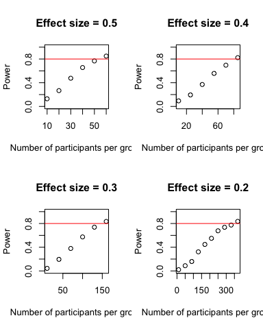
The results show that 80 percent power is exceeded with n = 60 at a moderate effect size, and the required n increases as the effect size decreases: n’s = 85, 160, and 370 at d’s = 0.4, 0.3, and 0.2, respectively.

Thus, two equal sized groups of between n = 60 and n = 370 each, will provide sufficient power to cover a moderate to small effect size.