Chapter 4 Analyses: Modeling the Time Course of Continuous Outcomes
The most basic feature of a longitudinal study is the time course or trajectory of the outcome measure (dependent variable or y). What is the trajectory of the typical subject? And how much do subjects differ from each other in their trajectory?
For this example we will need nlme (nonlinear
mixed-effect models) for it’s ability to explicitly model the
within-subject covariance structure.
library(tidyverse)
library(nlme)
The time course dataset contains simulated data on an outcome where, as the result of an intervention, there is reason to expect group differences in the time course and, over and above these, subject-level differences within each group. The dataset is intended to represent a study of wives from 50 heterosexual married couples, randomly assigned to a 16-week marital therapy treatment condition ( n = 25) or a 16-week wait-list condition ( n = 25). In the treatment group each wife completed a web diary each week on the evening prior to the day of the therapy session, and in the control group each wife completed a web diary on a fixed day each week.
time <- read_csv('time.csv') |>
  mutate(treatment = as.factor(treatment),
         id = as.factor(id))
## Rows: 800 Columns: 5
## ── Column specification ───────────────────────────────────────────────────────────────────────
## Delimiter: ","
## dbl (5): id, time, time01, intimacy, treatment
##
## ℹ Use `spec()` to retrieve the full column specification for this data.
## ℹ Specify the column types or set `show_col_types = FALSE` to quiet this message.# peak at the data
time |>
ggplot(aes(x = time01, y = intimacy)) +
geom_line(aes(linetype = treatment)) +
facet_wrap(~id) +
labs(x = "", y = "",
subtitle = "Panel plots of the 16-week trajectory of intimacy for each subject in the control and treatment groups") +
theme(legend.position = "top")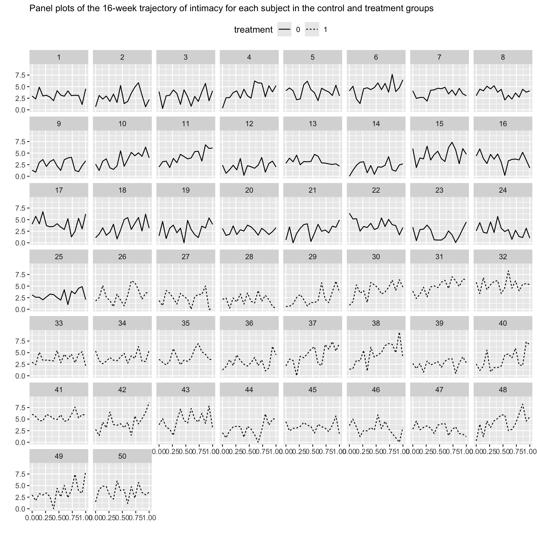
Model
A random effects model with fixed terms for time and treatment group, and their interaction, along with random intercepts and slopes per subject. The within-subject covariance matrix with AR(1) errors.
A central concern in modeling intensive longitudinal data is to estimate the population variances and covariances of the fixed effects. These allow us to know how much subjects differ from one another within the treatment and control groups, and, in case of the intercept–slope covariance, whether there is any tendency for subjects with larger or smaller intercepts (i.e., starting levels) to have larger or smaller slopes.
The random effects for the intercept and slope are termed upper-level or between-subjects random effects; there are also lower-level or within-subjects random effects. These are the \(\epsilon_{ij}\)’s, and they capture the extent to which a wife’s intimacy on a given week deviates above or below the value predicted by her specific regression line. We assume the \(\epsilon_{ij}\)’s are strictly ordered in time with serial correlations. The simplest serial correlation is where the current error is a linear function of the previous error, plus a truly random \(v_{ij}\): \(\epsilon_{ij} = \rho \epsilon_{i-1, j} + v_{ij}\).
Ignoring autocorrelation in errors typically leads to estimates of fixed effects that have standard errors that are too small, leading to Type I errors.
linear growth model with AR(1) errors
lgmodel <- lme(
  fixed = intimacy ~ time01*treatment,
  data = time,
  random = ~time01 | id,
  correlation = corAR1())

summary(lgmodel)
## Linear mixed-effects model fit by REML
## Data: time
## AIC BIC logLik
## 2852 2895 -1417
##
## Random effects:
## Formula: ~time01 | id
## Structure: General positive-definite, Log-Cholesky parametrization
## StdDev Corr
## (Intercept) 0.828 (Intr)
## time01 1.376 -0.453
## Residual 1.301
##
## Correlation Structure: AR(1)
## Formula: ~1 | id
## Parameter estimate(s):
## Phi
## -0.0000366
## Fixed effects: intimacy ~ time01 * treatment
## Value Std.Error DF t-value p-value
## (Intercept) 2.899 0.207 748 14.00 0.0000
## time01 0.735 0.347 748 2.12 0.0345
## treatment1 -0.056 0.293 48 -0.19 0.8479
## time01:treatment1 0.921 0.491 748 1.88 0.0610
## Correlation:
## (Intr) time01 trtmn1
## time01 -0.599
## treatment1 -0.707 0.423
## time01:treatment1 0.423 -0.707 -0.599
##
## Standardized Within-Group Residuals:
## Min Q1 Med Q3 Max
## -2.624 -0.680 -0.019 0.643 2.446
##
## Number of Observations: 800
## Number of Groups: 50Plot results
time$predicted <- fitted(lgmodel)

time |>
  mutate(treatment = as.factor(treatment)) |>
  ggplot(aes(x = time01)) +
    geom_line(aes(y = intimacy, linetype = treatment)) +
    # compare to BLUE
    geom_smooth(aes(y = intimacy), method = "lm", formula = 'y ~ x', se = F,
                color = "black", linewidth = .5) +
    geom_line(aes(y = predicted), color = "blue") + # BLUP?
    facet_wrap(~id) +
    labs(x = "", y = "",
         subtitle = "Panel plots of the actual and predicted trajectory of intimacy for each subject") +
    theme(legend.position = "top")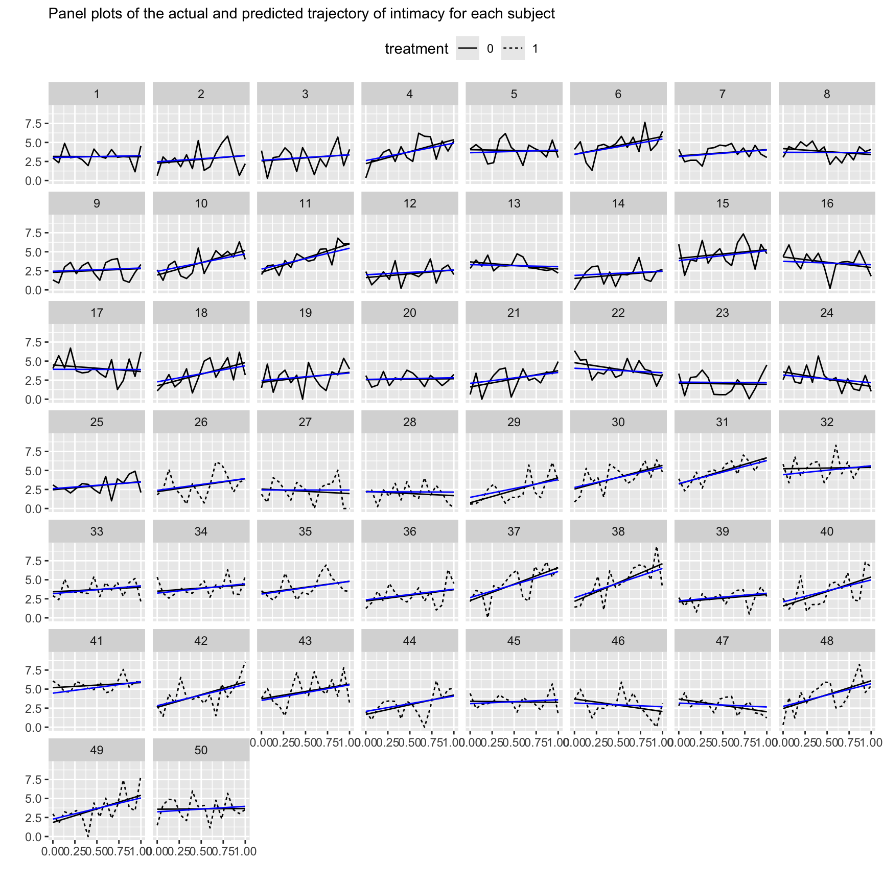
Compare estimates for treated and control
time |>
  mutate(treatment = as.factor(treatment)) |>
  ggplot(aes(x = time01, y = predicted)) +
    geom_line(aes(group = id)) + # BLUP?
    geom_smooth(aes(group = treatment),
                method = "lm", formula = 'y ~ x', se = F,
                linewidth = 2, color = "red") +
    facet_wrap(~treatment) +
    labs(x = "", y = "",
         subtitle = "Subject-specific regression lines for the control (left) and treatment (right) groups.
Average slope is shown in red") +
    theme(legend.position = "top")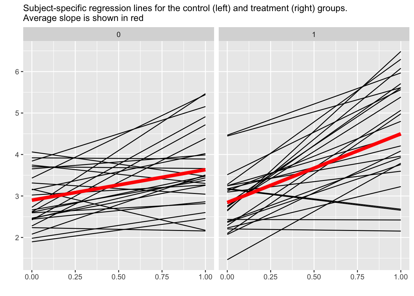
The fixed effects, can be thought of as the results for typical persons in the control and treatment groups, respectively. These fixed effects are represented by the red lines in this figure. The between-subject random effects are represented by the variability in individual regression lines from the group averages. The lower-level (within-subject) random effects are represented by the difference between the raw data and predicted slopes in the earlier figure above.
EB estimates
Percentiles of slope distributions of the control and treatment groups are shown below. There is substantial overlap between both distributions (this would be better shown by the relative advantage of the treatment group distribution over the control group: TBD)
rfx <- ranef(lgmodel) |>
  as_tibble(rownames = "id") |>
  rename(ebintercept = 2, ebslope = 3)

slopes <- coef(lgmodel) |>
  as_tibble(rownames = "id") |>
  select(id, slope = time01, interaction = 5) |>
  # add treatment indicator:
  left_join(
    distinct(select(time, id, treatment)) |>
      mutate(treatment = as.numeric(treatment == 1)),
    by = join_by(id)
  ) |>
  # group-specific slopes:
  mutate(slope = slope + treatment*interaction)

coefs.1 <- full_join(slopes, rfx, by = join_by(id)) |>
  select(id, treatment, ebintercept, ebslope, slope)

# Find percentiles for slope distribution for each group
coefs.1 |>
  group_by(treatment) |>
  reframe(
    p = fct_inorder(paste0(c(0.0, .05, .25, .50, .75, .95, 1.0)*100, "%")),
    qnt = quantile(slope, c(0.0, .05, .25, .50, .75, .95, 1.0))
  ) |>
spread(p, qnt)| treatment | 0% | 5% | 25% | 50% | 75% | 95% | 100% |
|---|---|---|---|---|---|---|---|
| 0 | -0.992 | -0.557 | -0.029 | 0.621 | 1.31 | 2.29 | 2.74 |
| 1 | -0.508 | -0.407 | 0.997 | 1.542 | 2.78 | 3.34 | 3.84 |